Mastering Excel: A Step-by-Step Guide to Using INDEX and MATCH

Quick Links

While the VLOOKUP function is good for finding values in Excel, it has its limitations. With a combination of the INDEX and MATCH functions instead, you can look up values in any location or direction in your spreadsheet.

The INDEX function returns a value based on a location you enter in the formula while MATCH does the reverse and returns a location based on the value you enter. When you combine these functions, you can find any number or text you need.

VLOOKUP Versus INDEX and MATCH

The difference between these functions and VLOOKUP is that VLOOKUP finds values from left to right. Hence the function’s name; VLOOKUP performs a vertical lookup.

Microsoft best explains the way VLOOKUP works :

There are certain limitations with using VLOOKUP—the VLOOKUP function can only look up a value from left to right. This means that the column containing the value you look up should always be located to the left of the column containing the return value.

Microsoft goes on to say that if your sheet isn’t set up in a way where VLOOKUP can help you find what you need, you can use INDEX and MATCH instead. So let’s look at how to use INDEX and MATCH in Excel.

INDEX and MATCH Function Basics

To use these functions together, it’s important to understand their purpose and structure.

The syntax for INDEX in Array Form is

    `INDEX(array, row_number, column_number)`

with the first two arguments required and the third optional.

INDEX looks up a position and returns its value. To find the value in the fourth row in the cell range D2 through D8, you would enter the following formula:

=INDEX(D2:D8,4)

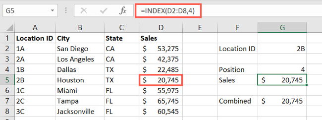
The result is 20,745 because that’s the value in the fourth position of our cell range.

For more details on the Array and Reference Forms of INDEX as well as other ways to use this function, take a look at our how-to for INDEX in Excel .

The syntax for MATCH is MATCH(value, array, match_type) with the first two arguments required and the third optional.

MATCH looks up a value and returns its position. To find the value in cell G2 in the range A2 through A8, you would enter the following formula:

=MATCH(G2,A2:A8)

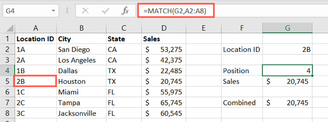
The result is 4 because the value in cell G2 is in the fourth position in our cell range.

For additional details on the match_type argument and other ways to use this function, take a look at our tutorial for MATCH in Excel .

How to Use INDEX and MATCH in Excel

Now that you know what each function does and its syntax, it’s time to put this dynamic duo to work. Below, we’ll use the same data as above for INDEX and MATCH individually.

You’ll place the formula for the MATCH function inside the formula of the INDEX function in place of the position to look up.

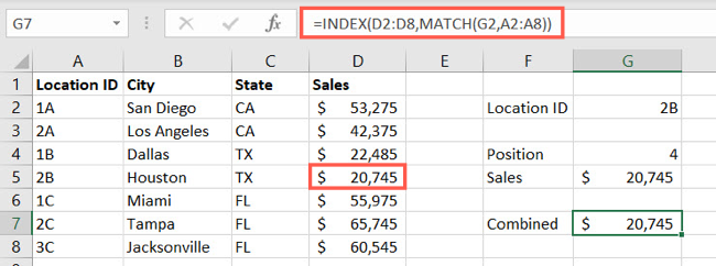
To find the value (sales) based on the location ID, you would use this formula:

=INDEX(D2:D8,MATCH(G2,A2:A8))

The result is 20,745. MATCH finds the value in cell G2 within the range A2 through A8 and provides that to INDEX which looks to cells D2 through D8 for the result.

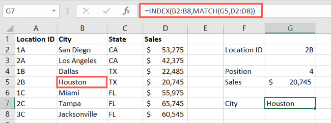
Let’s look at another example. We want to know which city has sales that match a certain amount. Using our sheet, you would enter this formula:

=INDEX(B2:B8,MATCH(G5,D2:D8))

The result is Houston. MATCH finds the value in cell G5 within the range D2 through D8 and provides that to INDEX which looks to cells B2 through B8 for the result.

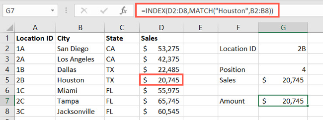
Here’s an example using an actual value instead of a cell reference. We’ll look for the value (sales) for a specific city with this formula:

=INDEX(D2:D8,MATCH(“Houston”,B2:B8))

In the MATCH formula, we replaced the cell reference containing the lookup value with the actual lookup value of “Houston” from B2 through B8 which gives us the result 20,745 from D2 through D8.

Be sure when you use the actual value to look up, rather than a cell reference, that you enclose it in quotes as shown here.

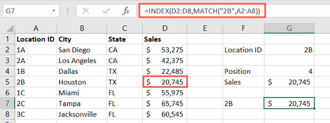
To obtain that same result by using the location ID instead of the city, we simply change the formula to this:

=INDEX(D2:D8,MATCH(“2B”,A2:A8))

Here we changed the MATCH formula to look up “2B” in the cell range A2 through A8 and provide that result to INDEX which then returns 20,745.

Basic functions in Excel like those that help you add numbers in cells or enter the current date are certainly helpful. But when you start adding more data and advancing your data entry or analysis needs, lookup functions like INDEX and MATCH in Excel can be quite useful.

Win11 Tips

Mastering Excel: A Step-by-Step Guide to Using INDEX and MATCH