Mastering Excel Data Insights: A Comprehensive Guide to Utilizing Pivot Tables

Pivot Tables are both incredibly simple and increasingly complex as you learn to master them. They’re great at sorting data and making it easier to understand, and even a complete Excel novice can find value in using them.

We’ll walk you through getting started with Pivot Tables in a Microsoft Excel spreadsheet.

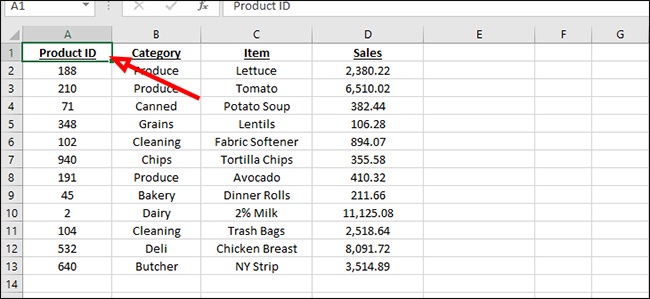
First, we’ll label the top row so that we can better organize our data once we apply the PivotTables in a later step.

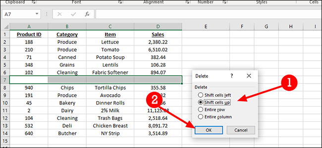
Before we continue, this is a good opportunity to get rid of any blank rows in your workbook. PivotTables work with blank cells, but they can’t quite understand how to proceed with a blank row. To delete, just highlight the row, right-click, choose “Delete,” then “Shift cells up” to combine the two sections.

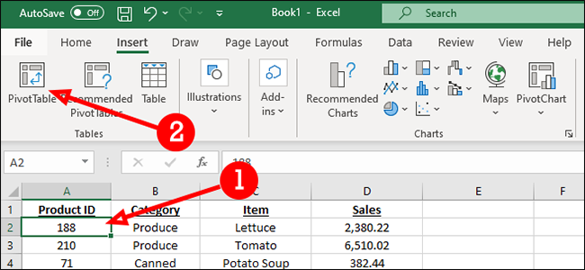
Click inside any cell in the data set. On the “Insert” tab, click the “PivotTable” button.

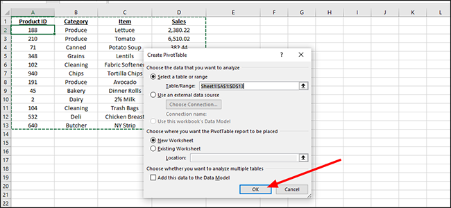
When the dialogue box appears, click “OK.” You can modify the settings within the Create PivotTable dialogue, but it’s usually unnecessary.

We have a lot of options here. The simplest of these is just grouping our products by category, with a total of all purchases at the bottom. To do this, we’ll just click next to each box in the “PivotTable Fields” section.

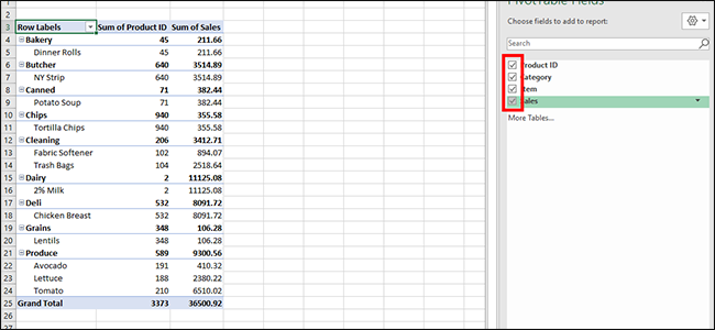
To make changes to the PivotTable, just click any cell inside the dataset to open the “PivotTable Fields” sidebar again.

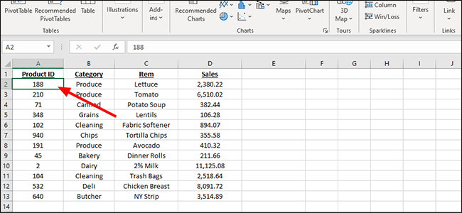
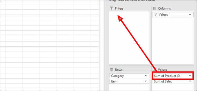
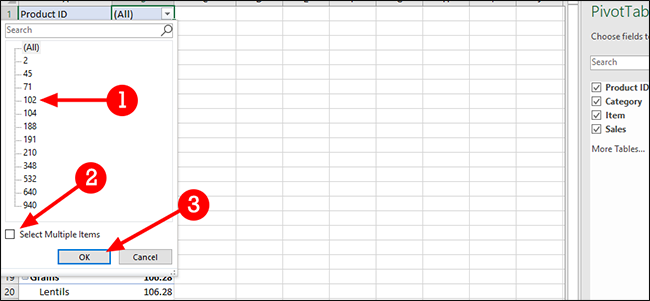
Once open, we’re going to clean up the data a bit. In our example, we don’t need our Product ID to be a sum, so we’ll move that from the “Values” field at the bottom to the “Filters” section instead. Just click and drag it into a new field and feel free to experiment here to find the format that works best for you.

To view a specific Product ID, just click the arrow next to “All” in the heading.

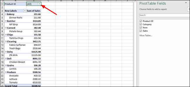
This dropdown is a sortable menu that enables you to view each Product ID on its own, or in combination with any other Product ID. To pick one product, just click it and then click “OK,’ or check the “Select Multiple Items” option to choose more than one Product ID.

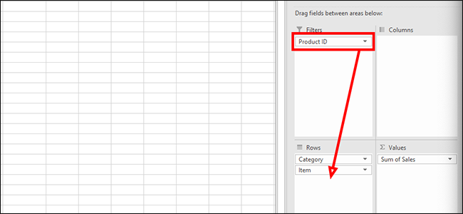
This is better, but still not ideal. Let’s try dragging Product ID to the “Rows” field instead.

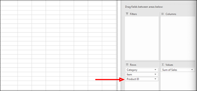
We’re getting closer. Now the Product ID appears closer to the product, making it a bit easier to understand. But it’s still not perfect. Instead of placing the Product ID below the product, let’s drag Product ID above Item inside the “Rows” field.

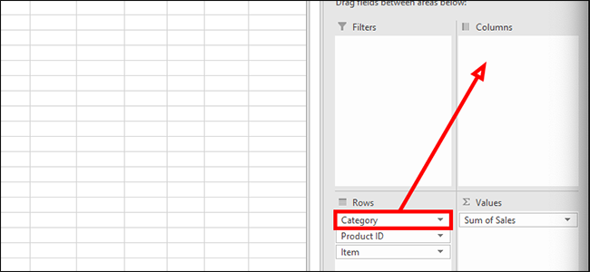
This looks much more usable, but perhaps we want a different view of the data. For that, we’re going to move Category from the “Rows” field to the “Columns” field for a different look.

We’re not selling a lot of dinner rolls, so we’ve decided to discontinue them and remove the Product ID from our report. To do that, we’ll click the arrow next to “Row Labels” to open a dropdown menu.

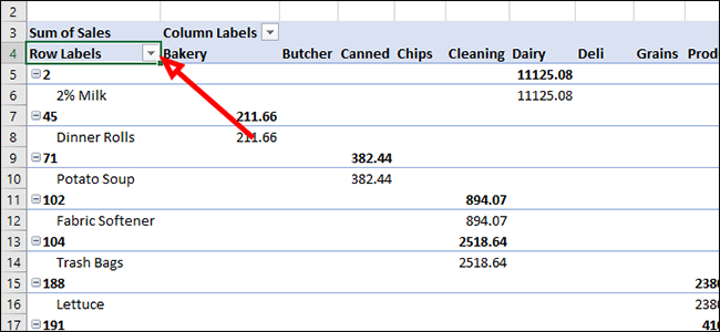
From the list of options, uncheck “45” which is the Product ID for dinner rolls. Unchecking this box and clicking “OK” will remove the product from the report.

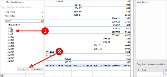
As you can see, there are a number of options to play with. How you display your data is really up to you, but with PivotTables, there’s really no shortage of options.

Also read: