Mastering Goal Seek Functionality in Microsoft Excel

Quick Links

• What Is Goal Seek in Excel?
• Goal Seek Examples

Have you ever had a financial goal you sought but weren’t exactly sure how to get there? Using Goal Seek in Microsoft Excel, you can determine what you need to accomplish your goal.

Maybe you want to save a certain amount of money in the next few years but aren’t sure how much you need to set aside each month. Or perhaps you want to take out a loan and know how much you can afford every month, but don’t know what interest rate to look for.

Goal Seek can help you with these types of calculations as well as others.

What Is Goal Seek in Excel?

Goal Seek is part of the What-If Analysis group built into Excel. It works with values you insert and a formula you enter to calculate those values. This means that a formula is necessary to use Goal Seek.

Related: 5 iPhone Apps to Keep Track of Your Investments

The tool is especially useful for the situations mentioned above such as savings, investments , and loans, but can be used in other scenarios as well. Once you obtain the results from the Goal Seek tool, you can simply view them or pop them into your sheet.

Goal Seek Examples

If you’re ready to give this nifty feature a try, let’s look at some example uses.

Goal Seek for Sales

For a simple way to get familiar with the tool, we’ll start with a basic example. We want to determine how many units of our product we need to sell to reach our goal. So, we have the current Quantity, Unit Price, and Total Sales as shown below.

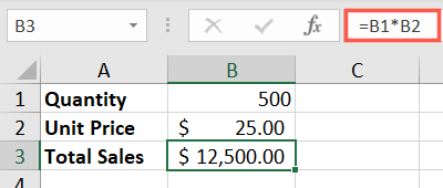
The Total Sales in cell B3 is a formula that multiples the Quantity by the Unit Price:

    `=B1*B2`

.

We want to find out how many units we must sell to reach our goal of $20,000 in total sales. For this, Goal Seek is ideal.

Go to the Data tab, click the What-If Analysis drop-down arrow, and select “Goal Seek.”

Epubor Ultimate for Win：Helps you read books anywhere, including the best eBook Converter + eBook DRM Removal functions.

In the small Goal Seek box, insert the following:

Set Cell: Enter the cell reference containing the formula you want to change. Remember, changing the formula shows us the input we need to reach our goal.

To Value: Enter the result you want. For us, this is 20,000.

By Changing Cell: Enter the reference for cell you want to adjust. For us, this is B1 for the Quantity.

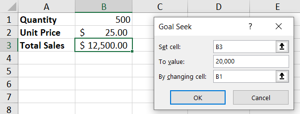
When you finish, click “OK.” The Goal Seek Status box shows a solution was found and you’ll see a preview in your spreadsheet.

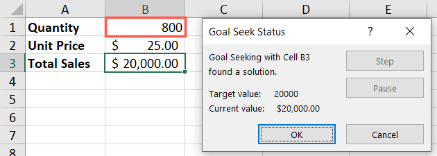
As you can see, we now know that we must sell 800 units of our product to reach our $20,000 goal. Click “OK” to apply the change to your sheet or “Cancel” to simply close the Goal Seek Status window.

Goal Seek for Loans

Another good way to use Goal Seek in Excel is for help with loans. You may have the loan amount, term in months, and payment you can afford, but want to know what interest rate you should seek. Because the Goal Seek tool works off of formulas, you can leave the interest rate cell blank and allow Goal Seek to fill it.

Related: How to Calculate a Loan Payment, Interest, or Term in Excel

Here we have the Loan Amount, Term, and Payment fields filled in. (You can ignore the payment amount displayed for now since the formula still needs the interest rate.) We have the formula for the PMT (Payment) function in cell B4:

    `=PMT(B3/12,B2,B1)`

.

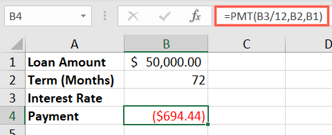
Select Data > What-If Analysis > Goal Seek and insert the following:

Set Cell: Enter the cell reference containing the formula you want to change. For us, this is B4.

To Value: Enter the result you want. For us, this is -800 because we can afford $800 monthly.

By Changing Cell: Enter the reference for cell you want to adjust. For us, this is B3 for the Interest Rate.

Excel uses a negative number for the payment when using the PMT function.

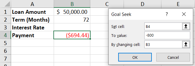
Click “OK” to see the results. It looks like we’ll try for a 4.77% annual interest rate for our loan.

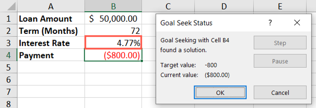
Select “OK” to apply the change to your sheet or “Cancel” to close the box.

Goal Seek for Savings

For one more example, you might have a savings goal you want to reach in a certain amount of time. We want to save $5,000 in 12 months, our bank offers 1.5% interest, and we need to know how much to deposit each month.

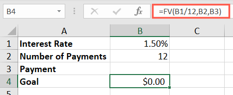
Here we have the Interest Rate and Number of Payments filled in. The Payment is blank because Goal Seek will enter it and the Goal is at $0 because the formula still needs the payment amount. We have the formula for the FV (Future Value) function in cell B4:

    `=FV(B1/12,B2,B3)`

.

Head back to Data > What-If Analysis > Goal Seek and insert the following:

Set Cell: Enter the cell reference containing the formula which is B4 in our example.

To Value: Enter the result you want. For our goal, this is 5000.

By Changing Cell: Enter the reference for cell you want to adjust which is B3 for the Payment.

Easy GIF Animator is a powerful animated GIF editor and the top tool for creating animated pictures, banners, buttons and GIF videos. You get extensive animation editing features, animation effects, unmatched image quality and optimization for the web. No other GIF animation software matches our features and ease of use, that’s why Easy GIF Animator is so popular.

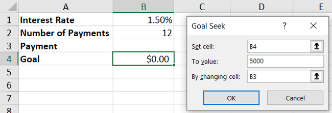
Click “OK” to view your results. We see that we need to save just over $413 per month for the next year to reach our $5,000 goal.

Excel uses a negative number for the payment when using the FV function.

Again, click “OK” to apply the change or “Cancel” to close the window.

When you need help figuring out how to reach your financial goal, pop open the Goal Seek tool in Excel. For more, take a look at how to use Excel’s built-in stocks feature .